Downloading and Installing R and RStudio
What is R?
R started as a free, open-source version of the statistical programming language S and S+. However, because it is open-source, many biologists have learned to use it and contributed to it and it is now the industry-standard statistical software. You can use it to do statistical analysis (not surprisingly), draw complex graphs, control other software, analyze DNA sequences and much more.
You may be very resistant to learning to program in a biology class, but biology is no longer an observational and descriptive science – it increasingly incorporates mathematical models and complex experimental design. Therefore, learning to use the tool, R, that has become essentially standard in the field, will benefit you greatly. It won’t come easy for many of you, but it’ll be worth it in the long run. Additionally, you’ll be able to put on your resume that you know a little bit about using it!
Because this is a biology class, we will only learn some very basic things about R. Primarily, we’ll use R to read in data, manipulate it a bit, and then make a graph and/or do a simple statistical test. It is likely that you have used Microsoft Excel in the past, and you will need to get a bit used to a different way of doing things. R doesn’t have a spreadsheet program to type and store data, so we will use Google Sheets for that. We will then tell R to grab the data from Google, manipulate it and output a graph or statistical result. Unlike Excel, we will be doing a bit of real programming in order to tell the computer what to do.
Choosing between RStudio and Posit Cloud
There are 2 convenient ways to use R. The first option is easiest and just requires you to sign up for a free online Posit Cloud account. Use the first option if you really aren’t interested in installing software on your computer. Also, use the first option if you have a chromebook or iPad if if, for some reason, you are unable to install all the steps for the second option. The second option is a more ‘standard’ way to use R, will require a bit more setup, but will be easier and faster in the long run.
- Online option. Use this option if you use a Chromebook, iPad or if you cannot install software to your computer.
- Use Posit Cloud. This provides full functionality in a convenient web app. To use this option, you’ll need to sign up for a free account. Although this option won’t require you to install anything, you’ll find that getting your files into and out of Posit Cloud more difficult than if you used the stand-alone apps in option 1. The user interface for Posit Cloud and RStudio are identical. You should be able to use Posit Cloud with an iPad, however getting files in and out is much more difficult, and you really should have a keyboard!
- Use this option if you use a Mac or a PC for which you can install software. Do all 3 of the following steps:
- Download and install a program called “git”.
- If you have a Mac:
- Go to the app launcher and search for and start “Terminal.app”. It is likely in your “Applications” folder in a subfolder called “Utilities”.
- Once Terminal is open, simply type “git –version”.
- If the computer responds with something like “git version 2.50.1 (Apple Git-155)”, then you have git and are ready to install R.
- If the computer responds with something like “command not found: git”, then your computer should prompt you with a dialog box to install it. You should just be able to follow directions.
- If you have a Windows PC:
- Go to this website to install Git
- Choose the “Windows” tab.
- Choose either of “Git for Windows/x64 Setup” or “Git for Windows/ARM64 Setup.” depending on your computer. You probably have an “x64” processor, so try that one. If it doesn’t work, check out this video to determine which type you have.
- Install git using the installer you just downloaded.
- If you have a Mac:
- Download and install R.
- Download and install RStudio Desktop. RStudio provides a nice user interface to R. R itself is much more difficult to use without such an interface, and RStudio is very good! Installation should be easy if you use Windows, MacOS, or (standard) Linux. If you use a Chromebook, you won’t be able to install it and will have to use the online option.
- Download and install a program called “git”.
Getting Started
Please follow along by actually doing the steps listed below. You can’t learn a new skill without practicing. Trust me, this will save you lots of frustration later on.
Open up the RStudio application or log on to your Posit Cloud account. You should see your window divided into 3 or 4 sections (Fig. 1).
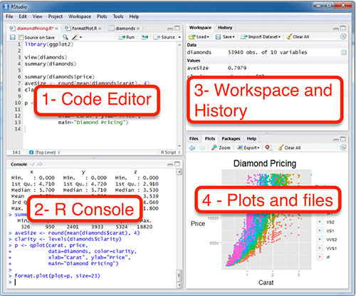
- Code editor. This is where you should write your code and save it.
Rconsole. This is whereRactually does its work. You will usually be able to ignore this section and just observe it for its output. That output will give you information that may help you debug your code.- Workspace and history. You will usually ignore this as well, however it can be useful for making sure that your data is read in properly.
- Plots and files. When you draw a graph, this is where it will appear. This pane can also be used for getting ‘help’ on an
Rcommand. You can also see files in your project here.
R File types
The simplest R files are called “R script” files that list, in order, the commands to execute. We will be using a slightly more complex file called ‘R markdown’ which allows us to mix computer R code with comments and explanations. It also allows us to produce a single finished document with all the figures integrated. These R markdown documents always have a file extension of “.Rmd”
Important note It is possible to run R one command at a time, but it is much better to save your commands in a file. This will allow you to re-run the code easily if you decide to change anything, or if your underlying data changes.
Getting Started – loading an R Markdown file
- Download the b40r project into Rby doing the following:
- If you are using Posit Cloud, make sure you are in a workspace, and then on the right, choose “New Project” and then “New Project from Git Repository”, then type or copy “https://github.com/senanu/b40r.git”
- If you are using RStudio on your own computer, go to File>New Project>Version Control>Git and type or copy “https://github.com/senanu/b40r.git” into the dialog. In the “create project as subdirectory of” box, choose a place (folder/directory) on your computer where you’d like to save everything.
- In the bottom-right pane, select the “Files” tab. You should see a list of files and directories (folders), starting with a directory called “.github”. All of the R Markdown files you need for this class will be located in the “R” directory.
- Click that “R” directory, and then click the link to “intro_to_rstudio.Rmd”.
- The file should open in the top-left pane.
- You will probably be given a yellow warning that a package called ‘rmarkdown’ and ‘knitr’ are required but not installed. Click “install” on the yellow banner. It will install on the web server, not on your computer.
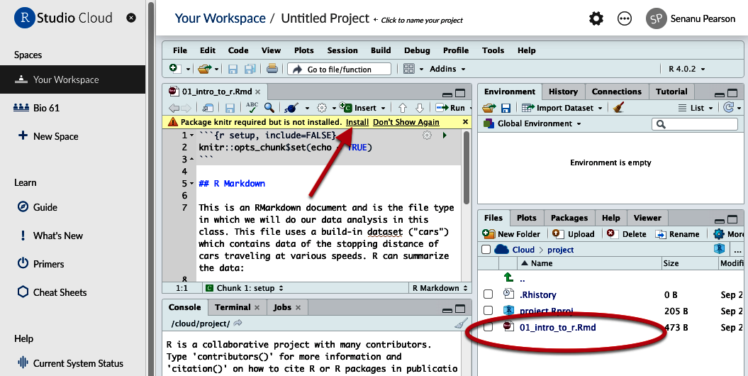
Figure 5. Location of uploaded file and Message to install Knitr
For each lab:
- Use the following steps for every lab in which we use R. This will help ensure that you have the newest files and that the data and objects you are working with are not accidentally saved from a previous lab.
- Use Git to “Pull” the latest version of the code onto your computer. Click the blue down arrow in the “Git” tab of the top right pane.
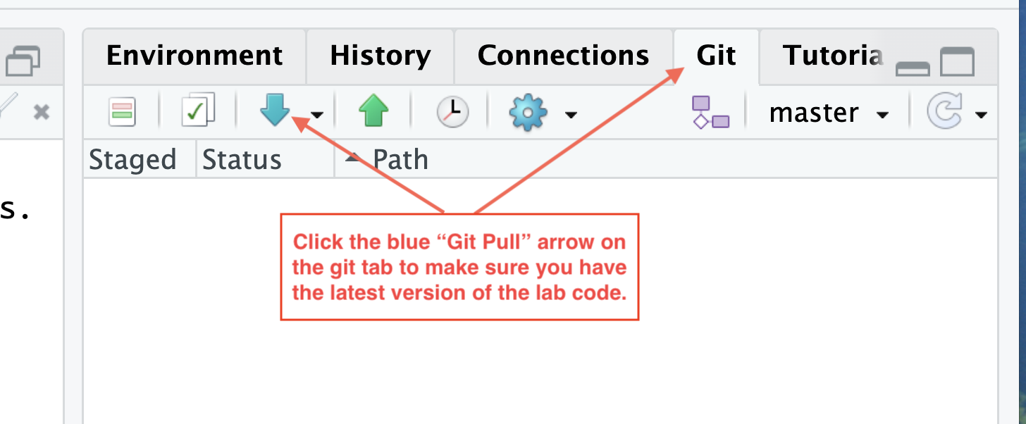
Git pull to make sure you have the most up-tp-date code - Go to the “Session” menu and select “Set Working Directory” and then “To source file location”.
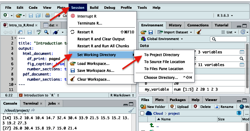
Figure 6. Setting the working directory - If there is a yellow banner asking you to install a new package, click “install”
- Clear the cache. Click on the knitting needles and yarn (‘knit’) and then select “Clear Knitr Cache…” (see screenshot below)
- Clear the environment. Click the ‘broom’ icon in the top-right panel within the “Environment” tab (see screenshot below)
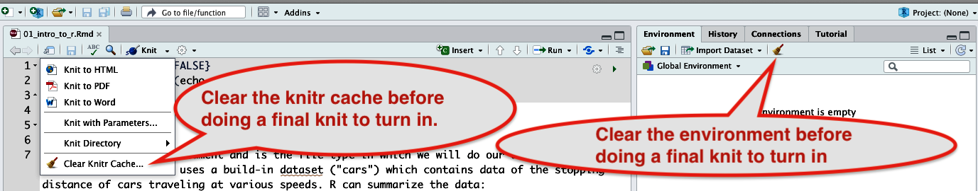
Figure 6. Setting the working directory - Go to the Session menu, and click “Restart R”
- Use Git to “Pull” the latest version of the code onto your computer. Click the blue down arrow in the “Git” tab of the top right pane.
You should now have the R Markdown file loaded into either RStudio or Posit Cloud.
Using R Markdown files
Now we will look at how to use the R Markdown files. As mentioned above, these files combine code with comments. The comments help us communicate in natural language what we are trying to do with code, in order for another person to be able to understand the code quickly. It is useful to include comments for your own code, because if you look at it a few weeks later, you may struggle to figure out what and why you did what you did.
The gray regions are called ‘code chunks’. These are the actual bits of code that R runs. The white areas are for comments and explanations. There are three main ways in which you can run the code.
- To run all of the code in the entire file, choose “Run” – “Run All” as shown below.
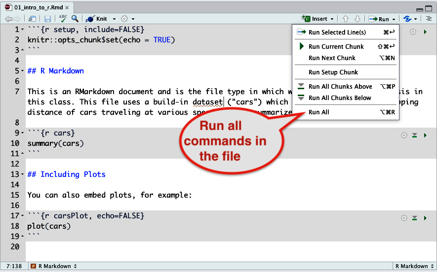
Figure 9. How to run all commands in a file. - You can run individual gray code chunks by clicking the little green arrow.
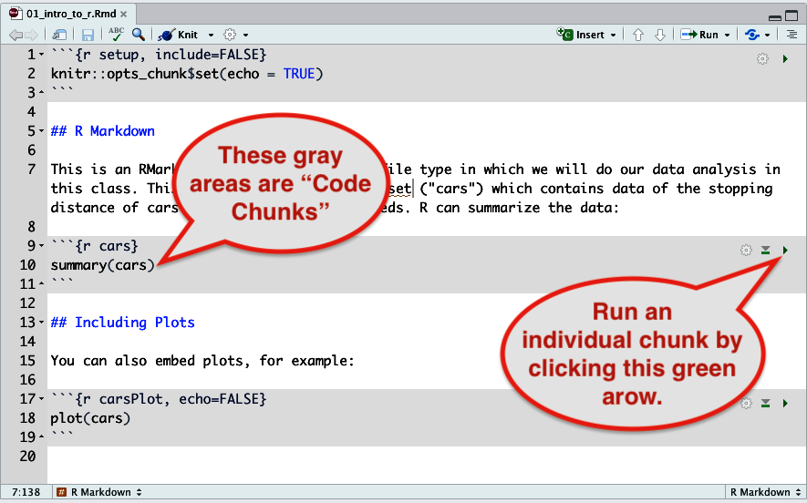
Figure 10. Click the green arrow to run a single code chunk (in gray) - You may run a single line by pressing “control-enter” (on a Windows PC) or “command-enter” (on a Mac).
Please become familiar with each of these 3 methods by using them on the gray parts of the file you have loaded.
You can view the Rmarkdown document in either “Source” or “Visual” mode, controlled by a button near the top left.
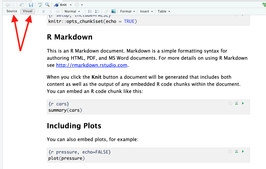
- In “Visual” mode, the document will look more like it’s final form. Headers will look like headers, bold will look bold, etc. I recommend that you use this mode most of the time.
- In “Source” mode, you will see all of the formatting codes and the document won’t be formatted. However, If you ever send me code, you must change it to “Source” mode before copying your code, because the formatting marks are important to include.
Before you move on, try toggling between the two modes to see how different the same document looks in each mode.
Knitting the documents
When you have finished a project, you would like to present a document that incorporates your code, output from your code (such as tables and figures) and text to explain what the analysis means. You need to “knit” the different parts of the file together.
- Click the little arrow next to the word ‘knit’.
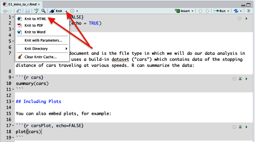
Figure 11. Knitting to produce an HTML document. Before you do this to turn in an HTML document, you must also select 'Clear Knitr Cache' from this same menu - Then click “Knit to HTML”. This will run all the code in the R Markdown file.
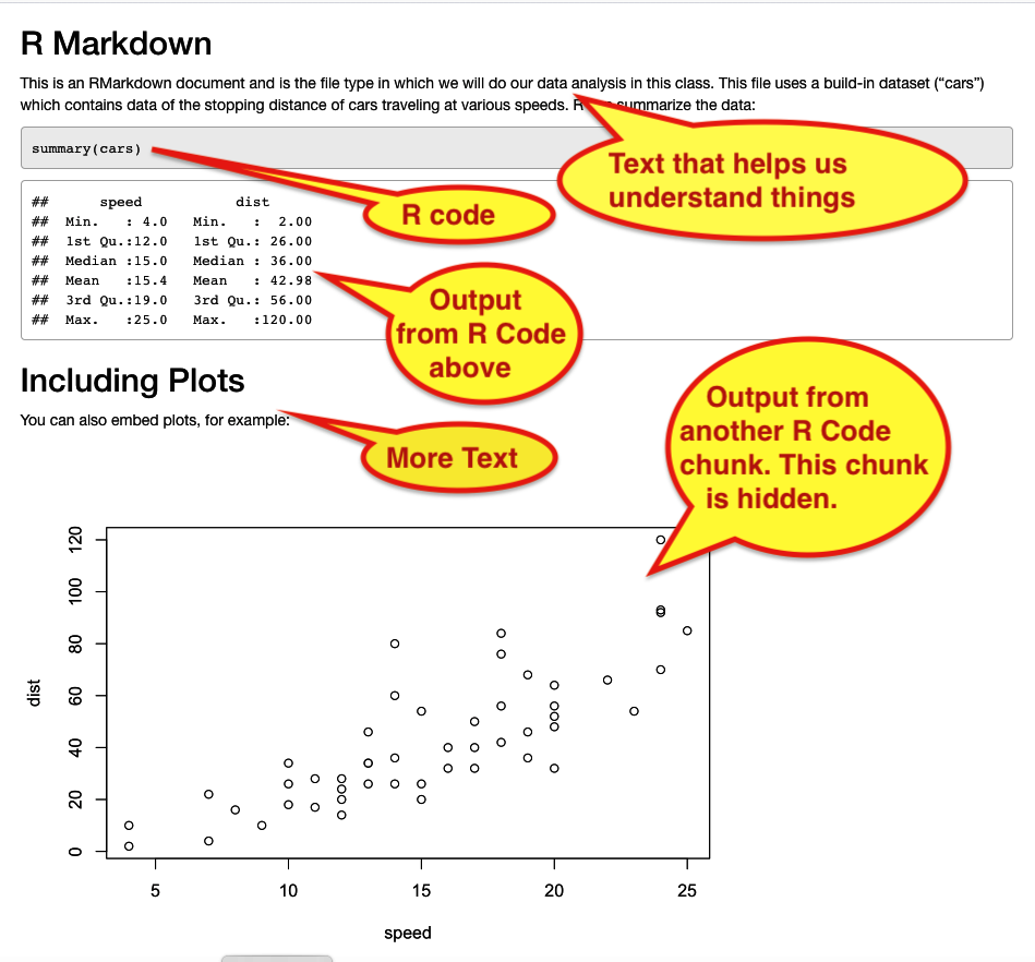
Figure 12. HTML output from knitting. - You will see an HTML file pop up. It has the text, code, and output (in this case, a graph), all ‘knitted’ together.
- in addition to the file that pops up, you will also see an .html file appear in the “Files” tab at the bottom-right.
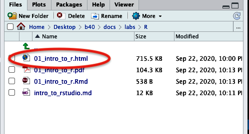
Figure 13. Knitted documents appear in lower right quadrant under 'Files' tab
If (when) you run into trouble
During the course of this semester, you will run into trouble and get stuck at some point. I can help!!! When this happens email me your entire .Rmd file either as an attachment or cut and paste it into your email. If you cut and paste, you must use “source” mode so that you also cut and paste all the formatting marks. If you don’t, you will simply be sending me a file that I cannot run, and I won’t be able to help you.
What to turn in
For this exercise, you only need to make a single change to the Rmd document. Usually, you will make changes in order to use your own data and analysis.
- By now, you should have accessed the git repository and have all of the Rmd files visible in the “Files” tab of the bottom-right pane in RStudio.
- Open the file “intro_to_rstudio.Rmd” and change the author name on the third line of the file to your own name.
- Save your file (you should do this periodically – it doesn’t save automatically like Google docs)
- Clear the knitr cache. To do so, click the triangle next to ‘Knit’ and select ‘Clear Knitr Cache…’.
Figure 14. Clear the knitr cache and the environment as preparation before you do a final knit to generate the HTML file to turn in. - Clear your environment. Click the broom in the top-right quadrant. After, it should say “Your environment is empty”.
- Knit the document that you loaded (“intro_to_rstudio.Rmd”). This will create a .html file in the directory you are working, and it may also open a browser window.
- Do one of the following:
- If you are using RStudio on your own computer, save the resulting .html file to turn in. You can save it directly from your browser “file” menu if you have it open.
- If you are using Posit Cloud, in the “Files” tab of the bottom-right pane, you should see “intro_to_rstudio.html” file. Check the box to the left of that file, then select the gear above, and choose “Export”. Save the file on your computer somewhere (it’ll probably go to the Downloads folder by default).
- Open the file in a browser (if it’s not already) to make sure it shows the results of your ‘data analysis’. If so, turn it in through Canvas.
It is important that you clear your knitr cache and your environment before you prepare your document to turn in. If you don’t, you may get some experimental code or data that you played with but didn’t work.